
Satellite positioning has become an essential part of modern surveying, but processing multiple GNSS sessions can quickly become repetitive. When several receivers observe simultaneously, manually creating every RTKLIB solution and then performing a network adjustment becomes both time-consuming and error-prone.
To simplify this workflow, I developed two Python applications that automate the entire process.
The first application performs batch processing of all available RINEX observations using RTKLIB’s rnx2rtkp.exe, while the second automatically builds and adjusts a complete relative GNSS network using Least Squares Adjustment.
This article presents the workflow together with a real test case.
1. Automatic RTKLIB Batch Processing
The first application searches a folder containing RINEX observation files and automatically computes every possible baseline.
Instead of manually selecting:
- Rover
- Base
- Navigation file
- Configuration
- Output filename
for each solution, the software performs everything automatically.
For a network containing several receivers this reduces processing time from several minutes to just a few seconds.
Each solution is stored as a standard RTKLIB .pos file that is immediately ready for network adjustment.
Typical features include:
- Automatic detection of RINEX observation files
- Automatic pairing of every station combination
- Support for mixed navigation files
- User-defined RTKLIB configuration
- Automatic organization of output files
2. Automatic Relative Network Adjustment
The second application reads every generated RTKLIB .pos file and performs a complete three-dimensional least-squares adjustment.
Unlike many simple baseline averaging approaches, the software treats every baseline as a vector observation and estimates the coordinates of all unknown stations simultaneously.
The program supports:
- Multiple fixed control stations
- Unlimited rover stations
- Unlimited baselines
- Full 3D vector adjustment
- Covariance propagation
- Error ellipse computation
- Statistical quality assessment
- Residual analysis
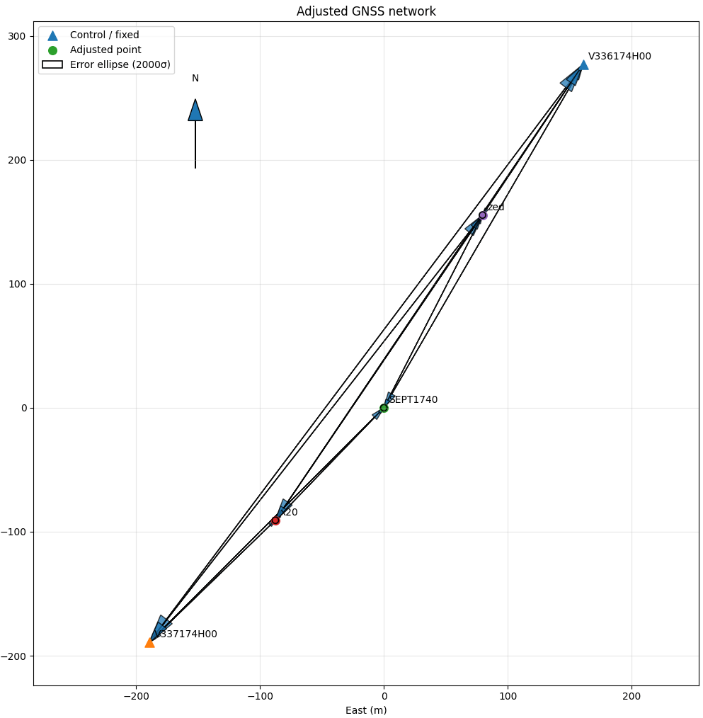
- Graphical visualization of the network before and after adjustment
The software can use either:
- the standard deviations reported by RTKLIB, or
- user-defined horizontal and vertical observation accuracies.
The adjustment report includes:
- Adjusted coordinates
- Coordinate covariance matrices
- Horizontal error ellipses
- Baseline residuals
- RMS statistics
- A-posteriori variance factor
- Degrees of freedom
- 95% confidence accuracies
Case Study
For testing, I processed a small GNSS network consisting of five receivers.
Fixed Control Stations
- V336174H00
- V337174H00
Unknown Stations
- SEPT1740
- x20
- zed
A total of 20 relative baseline solutions were generated automatically by the RTKLIB batch processor before being introduced into the network adjustment.
The adjustment was performed using predefined observation accuracies of:
- Horizontal σ = 10 mm
- Vertical σ = 20 mm
The resulting statistics were:
| Statistic | Value |
|---|---|
| Baselines processed | 20 |
| Unknown stations | 3 |
| Fixed stations | 2 |
| Degrees of freedom | 45 |
| A-posteriori variance factor | 0.594 |
| σ₀ | 0.7708 |
These values indicate a very consistent network with millimetre-level internal precision.
Coordinate Precision
The estimated coordinate precision for all unknown stations was approximately:
| Station | Horizontal (1σ) | 3D (1σ) |
|---|---|---|
| SEPT | 1.8 mm | 2.3 mm |
| x20 | 1.8 mm | 2.3 mm |
| zed | 1.8 mm | 2.3 mm |
The corresponding 95% horizontal confidence interval is approximately 3.6 mm.
Residual Analysis
One of the advantages of performing a network adjustment instead of relying on individual baseline solutions is the ability to evaluate consistency.
The adjustment computes residuals for every baseline, making it immediately possible to detect:
- inconsistent observations,
- poor GNSS sessions,
- multipath effects,
- incorrect fixed stations,
- or possible blunders.
In this dataset, most baseline RMS values remained below approximately 7 mm, indicating excellent agreement between independent observations.
Graphical Visualization
The software also produces graphical plots showing:
- the network before adjustment,
- the adjusted network,
- baseline vectors,
- station labels,
- and horizontal error ellipses.
These visualizations make it easy to inspect the network geometry and immediately identify weak areas.
Why Automate?
For projects involving many receivers, automation offers significant advantages:
- No manual RTKLIB processing
- No repetitive baseline creation
- Faster project completion
- Consistent processing parameters
- Objective statistical quality control
- Reliable least-squares adjustment
- Easy detection of problematic observations
Instead of processing dozens of baselines manually, the entire workflow—from RINEX files to the final adjustment report—can be completed in only a few clicks.
Future Development
Future versions will include additional capabilities such as:
- support for full covariance matrices from RTKLIB
- mixed static and kinematic observations
- automatic outlier detection and reweighting
- export to GIS and CAD formats
- network visualization in local and projected coordinate systems
- PDF reporting with adjustment statistics and graphical summaries
Test Equipment
To evaluate the complete workflow under real surveying conditions, the network was intentionally composed of receivers from different manufacturers and performance classes.
The two control stations (V336174H00 and V337174H00) were established using HEPOS Virtual Reference Station (VRS) observations, providing the fixed reference coordinates for the network adjustment.
The three rover receivers were:
- Septentrio Mosaic-X5 (SEPT)
- u-blox ZED-F9P (zed)
- u-blox X20P (x20)
Each rover was processed independently against the available observations, and all relative baselines between the control stations and the rover receivers—as well as rover-to-rover baselines—were automatically generated using the RTKLIB batch processor. The resulting solutions were then combined in a single least-squares network adjustment.
This heterogeneous test demonstrates that the workflow is not limited to a specific GNSS receiver manufacturer. It can seamlessly integrate high-end geodetic receivers such as the Septentrio Mosaic-X5 with low-cost multi-frequency receivers like the u-blox ZED-F9P and u-blox X20P, making it a practical solution for mixed-equipment surveying projects.
Conclusion
Python, combined with RTKLIB, provides a powerful environment for building customized GNSS processing tools. By automating both baseline computation and least-squares network adjustment, repetitive processing is eliminated while providing surveyors with rigorous statistical information about their observations.
The complete workflow demonstrates how open-source software and custom development can deliver professional-grade GNSS processing with millimetre-level precision for engineering and geodetic surveying applications.
